Intuition for Taylor Series (DNA Analogy)
Author: kalid
Go to Source
Your body has a strange property: you can learn information about the entire organism from a single cell. Pick a cell, dive into the nucleus, and extract the DNA. You can now regrow the entire creature from that tiny sample.
There’s a math analogy here. Take a function, pick a specific point, and dive in. You can pull out enough data from a single point to rebuild the entire function. Whoa. It’s like remaking a movie from a single frame.
The Taylor Series discovers the “math DNA” behind a function and lets us rebuild it from a single data point. Let’s see how it works.
Pulling information from a point
Given a function like f(x) = x2, what can we discover at a single location?
Normally we’d expect to calculate a single value, like f(4) = 16. But there’s much more beneath the surface:
- f(x) = Value of function at point x
- f'(x) = First derivative, or how fast the function is changing (the velocity)
- f”(x) = Second derivative, or how fast the changes are changing (the acceleration)
- f”'(x) = Third derivative, or how fast the changes in the changes are changing (acceleration of the acceleration)
- And so on
Investigating a single point reveals multiple, possibly infinite, bits of information about the behavior. (Some functions have an endless amount of data (derivatives) at a single point).
So, given all this information, what should we do? Regrow the organism from a single cell, of course! (Maniacal cackle here.)
Growing a Function from a point
Our plan is to grow a function from a single starting point. But how can we describe any function in a generic way?
The big aha moment: imagine any function, at its core, is a polynomial (with possibly infinite terms):
![]()
To rebuild our function, we start at a fixed point (c_0) and add in a bunch of other terms based on the value we feed it (like c_1x). The “DNA” is the values c_0, c_1, c_2, c_3 that describe our function exactly.
Ok, we have a generic “function format”. But how do we find the coefficients for a specific function like sin(x) (height of angle x on the unit circle)? How do we pull out its DNA?
Time for the magic of 0.
Let’s start by plugging in the function value at x=0. Doing this, we get:

Every term vanishes except c_0, which makes sense: the starting point of our blueprint should be f(0). For f(x) = sin(x), we can work out c_0 = sin(0) = 0. We have our first bit of DNA!
Getting More DNA
Now that we know c_0, how do we isolate c_1 in this equation?
![]()
Hrm. A few ideas:
-
Can we set x = 1? That gives f(1) = c_0 + c_1(1) + c_2(12) + c_3(13) + ·s . Although we know c_0, the other constants are summed together. We can’t pull out c_1 by itself.
-
What if we divide by x? This gives:

Then we can set x=0 to make the other terms disappear… right? It’s a nice idea, except we’re now dividing by zero.
Hrm. This approach is really close. How can we almost divide by zero? Using the derivative!
If we take the derivative of the blueprint of f(x), we get:
![]()
![]()
Every power gets reduced by 1 and the c_0, a constant value, becomes zero. It’s almost too convenient.
Now we can isolate c_1 using our x=0 trick:

In our example, sin'(x) = cos(x) so in our example: f'(0) = sin'(0) = cos(0) = 1 = c_1
Yay, one more bit of DNA! This is the magic of the Taylor series: by repeatedly applying the derivative and setting x = 0, we can pull out the polynomial DNA.
Let’s try another round:
![]()
After taking the second derivative, the powers are reduced again. The first two terms (c_0 and c_1x) disappear, and we can again isolate c_2 by setting x=0:

For our sine example, sin” = -sin, so:

or c_2 = 0.
As we keep taking derivatives, we’re performing more multiplications and growing a factorial in front of each term (1!, 2!, 3!).
The Taylor Series for a function around point x=0 is:

(Technically, the Taylor series around the point x=0 is called the MacLaurin series.)
The generalized Taylor series, extracted from any point a is:

The idea is the same. Instead of our regular blueprint, we use:
![]()
Since we’re growing from f(a), we can see that f(a) = c_0 + 0 + 0 + dots = c_0. The other coefficients can be extracted by taking derivatives and setting x = a (instead of x =0).
Example: Taylor Series of sin(x)
Plugging in derivatives into the formula above, here’s the Taylor series of sin(x) around x = 0:

And here’s what that looks like:
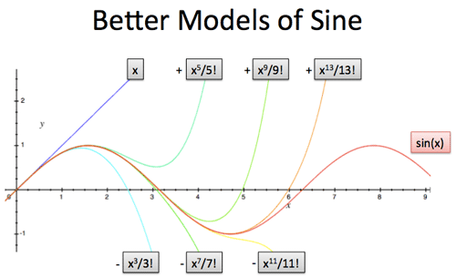
A few notes:
1) Sine has infinite terms
Sine is an infinite wave, and as you can guess, needs an infinite number of terms to keep it going. Simpler functions (like f(x) = x2 + 3) are already in their “polynomial format” and don’t have infinite derivatives to keep the DNA going.
2) Sine is missing every other term
If we repeatedly take the derivative of sine at x = 0 we get:
![]()
with values:

Ignoring the division by the factorial, we get the pattern:
![]()
So the DNA of sine is something like [0, 1, 0, -1] repeating.
3) Different starting positions have different DNA
For fun, here’s the Taylor series of sin(x) starting at x =π (link):

A few notes:
-
The DNA is now something like [0, -1, 0, 1]. The cycle is similar, but the starting value has changed since we’re starting at x=π.
-
Written as calculated numbers, the denominators 1, 6, 120, 5040 look strange. But they’re just every other factorial: 1! = 1, 3! = 6, 5! =120, 7! = 5040. In general, the Taylor series can have gnarly denominators.
- The O(x12) term means there are other components of order (power) x12 and higher. Because sin(x) has infinite derivatives, we have infinite terms and the computer has to cut us off somewhere. (You’ve had enough Tayloring for today, buddy.)
Application: Function Approximations
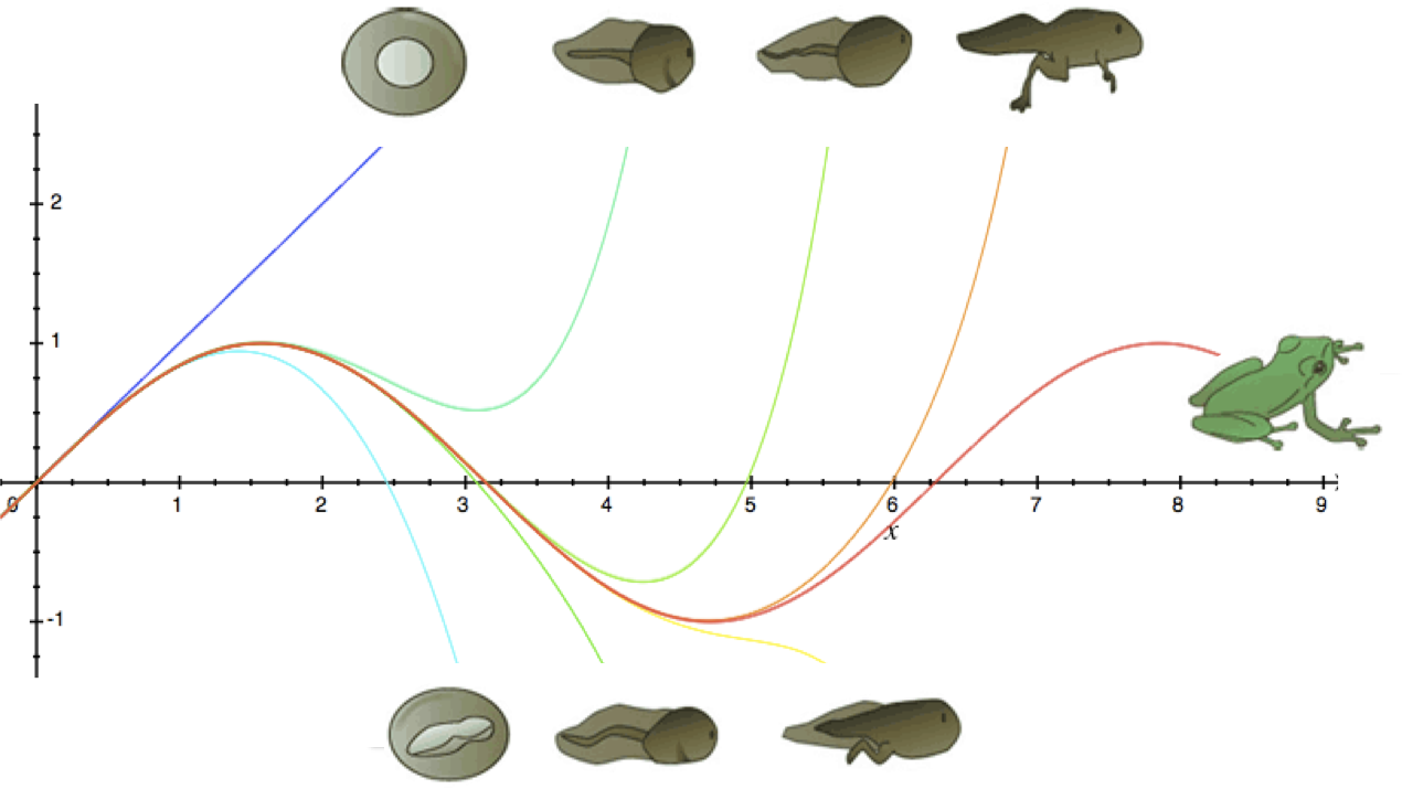
A popular use of Taylor series is getting a quick approximation for a function. If you want a tadpole, do you need the DNA for the entire frog?

The Taylor series has a bunch of terms, typically ordered by importance:

- c_0 = f(0), the constant term, is the exact value at the point
- c_1 = f'(0)x, the linear term, tells us what speed to move from our point
- c_2= frac(f”(0))(2!)x2, the quadratic term, tells us how much to accelerate away from our point
- and so on
If we only need a prediction for a few instants around our point, the initial position & velocity may be good enough:

If we’re tracking for longer, then acceleration becomes important:
![]()
![]()
As we get further from our starting point, we need more terms to keep our prediction accurate. For example, the linear model sin(x) = x is a good prediction around x=0. As we get further out, we need to account for more terms.
Similarly, ex sim 1 + x works well for small interest rates: 1% discrete interest is 1.01 after one time period, 1% continuous interest is a tad higher than 1.01. As time goes on, the linear model falls behind because it ignores the compounding effects.
Application: Comparing Functions
What’s a common application of DNA? Paternity tests.
If we have a few functions, we can compare their Taylor series to see if they’re related.
Here’s the expansions of sin(x), cos(x), and ex:
![displaystyle{ sin x = x - frac{x^3}{3!} + frac{x^5}{5!} - dots xrightarrow{DNA} [0, 1, 0 -1, dots] } displaystyle{ sin x = x - frac{x^3}{3!} + frac{x^5}{5!} - dots xrightarrow{DNA} [0, 1, 0 -1, dots] }](https://betterexplained.com/wp-content/plugins/wp-latexrender/pictures/b5ea819a6da480914052558967c23ba2.png)
![]()
![displaystyle{ e^x = 1 + x + frac{x^2}{2!} + frac{x^3}{3!} + dots xrightarrow{DNA} [1, 1, 1, 1, dots] } displaystyle{ e^x = 1 + x + frac{x^2}{2!} + frac{x^3}{3!} + dots xrightarrow{DNA} [1, 1, 1, 1, dots] }](https://betterexplained.com/wp-content/plugins/wp-latexrender/pictures/b40225aedb74d8648649c58ecb22cfa7.png)
There’s a family resemblence in the sequences, right? Clean powers of x divided by a factorial?
One problem is the sequence for ex has positive terms, while sine and cosine alternate signs. How can we link these together?
Euler’s great insight was realizing an imaginary number could swap the sign from positive to negative:
![{begin{aligned}e^{ix}&=1+ix+{frac {(ix)^{2}}{2!}}+{frac {(ix)^{3}}{3!}}+{frac {(ix)^{4}}{4!}}+{frac {(ix)^{5}}{5!}}+{frac {(ix)^{6}}{6!}}+{frac {(ix)^{7}}{7!}}+{frac {(ix)^{8}}{8!}}+cdots \[8pt]&=1+ix-{frac {x^{2}}{2!}}-{frac {ix^{3}}{3!}}+{frac {x^{4}}{4!}}+{frac {ix^{5}}{5!}}-{frac {x^{6}}{6!}}-{frac {ix^{7}}{7!}}+{frac {x^{8}}{8!}}+cdots \[8pt]&=left(1-{frac {x^{2}}{2!}}+{frac {x^{4}}{4!}}-{frac {x^{6}}{6!}}+{frac {x^{8}}{8!}}-cdots right)+ileft(x-{frac {x^{3}}{3!}}+{frac {x^{5}}{5!}}-{frac {x^{7}}{7!}}+cdots right)\[8pt]&=cos x+isin x.end{aligned}} {begin{aligned}e^{ix}&=1+ix+{frac {(ix)^{2}}{2!}}+{frac {(ix)^{3}}{3!}}+{frac {(ix)^{4}}{4!}}+{frac {(ix)^{5}}{5!}}+{frac {(ix)^{6}}{6!}}+{frac {(ix)^{7}}{7!}}+{frac {(ix)^{8}}{8!}}+cdots \[8pt]&=1+ix-{frac {x^{2}}{2!}}-{frac {ix^{3}}{3!}}+{frac {x^{4}}{4!}}+{frac {ix^{5}}{5!}}-{frac {x^{6}}{6!}}-{frac {ix^{7}}{7!}}+{frac {x^{8}}{8!}}+cdots \[8pt]&=left(1-{frac {x^{2}}{2!}}+{frac {x^{4}}{4!}}-{frac {x^{6}}{6!}}+{frac {x^{8}}{8!}}-cdots right)+ileft(x-{frac {x^{3}}{3!}}+{frac {x^{5}}{5!}}-{frac {x^{7}}{7!}}+cdots right)\[8pt]&=cos x+isin x.end{aligned}}](https://betterexplained.com/wp-content/plugins/wp-latexrender/pictures/cf7a66a77e3612eab7cde26914da2c7e.png)
Whoa. Using an imaginary exponent and separating into odd/even powers reveals that sine and cosine are hiding inside the exponential function. Amazing.
Although this proof of Euler’s Formula doesn’t show why the imaginary number makes sense, it reveals the baby daddy hiding backstage.
Appendix: Assorted Aha! Moments
1) Relationship to Fourier Series
The Taylor Series extracts the “polynomial DNA” and the Fourier Series/Transform extracts the “circular DNA” of a function. Both see functions as built from smaller parts (polynomials or exponential paths).
2) Does the Taylor Series always work?
This gets into mathematical analysis beyond my depth, but certain functions aren’t easily (or ever) approximated with polynomials.
Notice that powers like x2, x3 explode as x grows. In order to have a slow, gradual curve, you need an army of polynomial terms fighting it out, with one winner barely emerging. If you stop the train too early, the approximation explodes again.
For example, here’s the Taylor Series for ln(1 + x). The black line is the curve we want, and adding more terms, even dozens, barely gets us accuracy beyond x=1.0. It’s just too hard to maintain a gentle slope with terms that want to run hog wild.
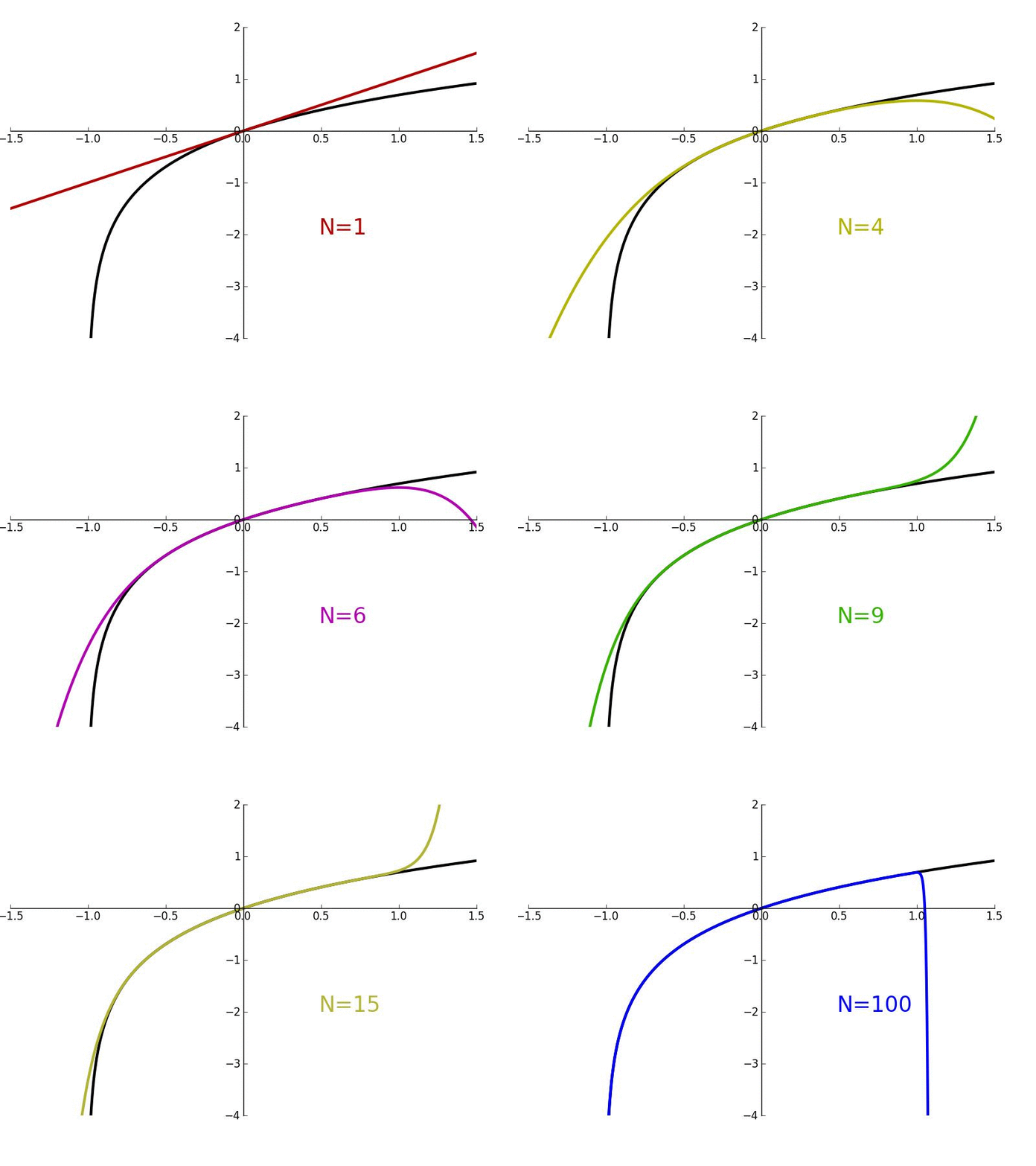
In this case, we only have a radius of convergence where the approximation stays accurate (such as around |x| < 1).
3) Turning geometric to algebraic definitions
Sine is often defined geometrically: the height of a line on a circular figure.
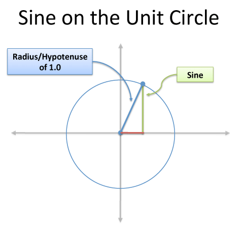
Turning this into an equation seems really hard. The Taylor Series gives us a process: If we know a single value and how it changes (the derivative), we can reverse-engineer the DNA.
Similarly, the description of ex as “the function with its derivative equal to the current value” yields the DNA [1, 1, 1, 1], and polynomial f(x) = 1 + frac(1)(1!)x + frac(1)(2!)x2 + frac(1)(3!)x3 + dots . We went from a verbal description to an equation.
Phew! A few items to ponder.
Happy math.
